
Click here to see other posts about XRD
Our XRD interpretation includes:
1. Phase determination
2. Determination of diffracted planes
3- Calculation of crystalline size and microstrain
4- Whatever your request
Its cost is only 12$
Payment Upon Completion

Send your patterns...
X-ray diffraction (XRD) is a technique used in materials science for determining the atomic and molecular structure of a material. This is done by irradiating a sample of the material with incident X-rays and then measuring the intensities and scattering angles of the X-rays that are scattered by the material. The intensity of the scattered X-rays are plotted as a function of the scattering angle, and the structure of the material is determined from the analysis of the location, in angle, and the intensities of scattered intensity peaks. Beyond being able to measure the average positions of the atoms in the crystal, information on how the actual structure deviates from the ideal one, resulting for example from internal stress or from defects, can be determined.

The diffraction of the X-rays, that is central to the XRD method, is a subset of the general X-ray scattering phenomena. XRD, which is generally used to mean can wide-angle X-ray diffraction (WAXD), falls under several methods that use the elastically scattered X-ray waves. Other elastic scattering based X-ray techniques include small angle X-ray scattering (SAXS), where the X-rays are incident on the sample over the small angular range of 0.1-100typically). SAXS measures structural correlations of the scale of several nanometers or larger (such as crystal superstructures), and X-ray reflectivity that measures the thickness, roughness, and density of thin films. WAXD covers an angular range beyond 100.
CITE THIS VIDEO | REPRINTS AND PERMISSIONS
JoVE Science Education Database. Materials Engineering. X-ray Diffraction. JoVE, Cambridge, MA, (2020).
PRINCIPLES
Relationship between diffracted peak positions and crystal structure:
When light waves of sufficiently small wavelength are incident upon a crystal lattice, they diffract from the lattice points. At certain angles of incidence, the diffracted parallel waves constructively interfere and create detectable peaks in intensity. W.H. Bragg identified the relationship illustrated in Figure 1 and derived a corresponding equation:
nλ = 2dhkl sin θ [1]
Here λ is the wavelength of the X-rays used, dhkl is the spacing between a particular set of planes with (hkl) Miller indices*, and θ is the angle of incidence at which a diffraction peak is measured. Finally, n is an integer that represents the ‘harmonic order’ of the diffraction. At n=1, for example, we have the first harmonic, meaning that the path of X-rays diffracted through the crystal (equivalent to 2dhkl sin ) is exactly 1λ, while at n=2, the diffracted path is 2λ. We can typically assume n=1, and, in general, n=1 for θ < sin-1(2λ/dh’k’l’), where h’k’l’ are the Miller indices of the planes that show the first peak (at the lowest 2θ value) in a diffraction experiment. Miller indices are a set of three integers that constitute a notation system for identifying directions and planes within crystals. For directions, the [h k l]Miller indices represent the normalized difference in the respective x, y and z coordinates (in a Cartesian coordinate system) of two points along the direction. For planes, the Miller indices (h k l) of a plane are simply the h k l values of the direction perpendicular to the plane.
In a typical XRD experiment in reflection mode, the X-ray source is fixed in position and the sample is rotated with respect to the X-ray beam over θ. A detector picks up the diffracted beam and has to keep up with the sample rotation by rotating at twice the rate (i.e. for a given sample angle of θ, the detector angle is 2θ). The geometry of the experiment is schematically shown in Figure 1.
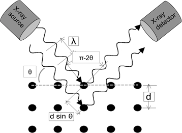
Figure 1: Illustration of Bragg’s Law.
When a peak in intensity is observed, equation 1 is necessarily satisfied. Consequently, we can calculate d-spacings based on the angles at which these peaks are observed. By calculating the d-spacings of multiple peaks, the crystal class and the crystal structure parameters material sample can be identified using a database such as the Hanawalt Search Manual or database libraries available with the XRD software being used.
We will be assuming that the sample being investigated is not a single crystal. If the sample were a single crystal with a particular (h*k*l*) plane parallel to the sample surface, it would need to be rotated until the Bragg condition for the (h*k*l*) is satisfied in order to see a peak in diffracted intensity (for n=1) with potentially higher harmonic (h*k*l*)peaks (e.g. for n=2) also detectable at higher angles. At all other angles there would be no peaks in a single crystal sample. Instead, let’s assume that the sample is either polycrystalline or that it is a powder, with a statistically significant number of crystalline grains or powder particles illuminated by the incident X-ray beam. Under this assumption, the sample consists of randomly oriented grains, with a similar statistical probability for all possible lattice planes to diffract.
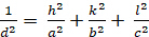
The relationships between the dhkl and the unit cell parameters are shown below in Equations 2-7 for the 7 crystal classes, cubic, tetragonal, hexagonal, rhombohedral, orthorhombic, monoclinic and triclinic. The unit cell parameters consist of lengths of(a,b,c) and the angles between (α, β, γ) the edges of the unit cells for the 7 crystal classes (Figure 1x shows the example of one of the crystal classes: the tetragonal structure where a=b≠c, and α=β=γ=900). Using multiple diffracted peak positions (i.e. several distinct dhkl values), the values of the unit cell parameters can be solved uniquely.
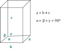
Figure 2: The tetragonal structure as one of the seven crystal classes.
Cubic (a = b = c; α = β = γ = 900):
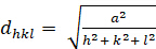
[2]
Tetragonal (a = b ≠ c; α = β = γ = 900):

[3]
Hexagonal (a = b ≠ c; α = β = 900; γ = 1200):
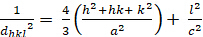
[4]
Orthorhombic (a ≠ b ≠ c; α = β = γ = 900):
[5]
Rhombohedral (a = b ≠ c; α = β = γ = 900):
[6]
Monoclinic (a ≠ b ≠ c; α = γ = 900≠ β):
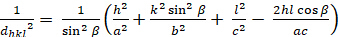
[7]
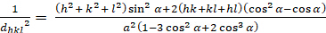
Triclinic (a ≠ b ≠ c; α ≠ β ≠ γ ≠ 900):

[8]
Relationship between diffracted peak intensities and crystal structure:
Next we examine the factors that contribute to the intensity in an XRD pattern. The factors can be broken down as 1) the contribution to scattering that results directly from the unique structural aspects of the material (the specific types and locations of scattering atoms in the structure) and 2) those that are not specific to the material. In the former, there are two factors: the ‘absorption factor’ and the ‘structure factor’. The absorption factor primarily depends on the ability of the material to absorb X-rays on their way in and out. This factor does not have a θ dependence as long as the samples are not thin (the sample should be > 3 times thicker than the attenuation length of the X-rays). In other words, the contribution by the absorption factor to the intensity of different peaks is constant. The ‘structure factor’ directly affects the intensity of specific peaks as a direct result of the structure. The remaining factors, the ‘multiplicity’, which accounts for all the planes that belong to the same family because they are symmetrically related, and the ‘Lorentz-Polarization’ factor, which comes from the geometry of the XRD experiment, also affect the relative intensity of the peaks but they are not specific to a material and can easily be accounted for with analytical expressions (i.e. XRD analysis software can remove them with analytical functions).
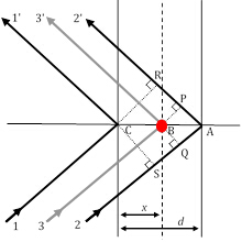
Figure 3: Three diffraction ray paths, of which rays 11′ and 22′ satisfy the Bragg condition, while ray 33′ results from scattering by an atom (red circle) at an arbitrary position.
As the only factor that carries the unique structural contribution of a material to the relative intensities of XRD peaks, the structure factor is very important and requires a closer look. In Figure 2, let us assume that the 1st order Bragg diffraction condition (remember, that this corresponds to n=1) is satisfied between ray11′ and ray22′ which are scattered on two atomic planes in the h00 direction (using the Miller indices notation described earlier) separated by a distance d. Under this condition, the difference in path length between ray11′ and ray22′ is δ(22′-11′) = SA + AR = λ. The phase shift between the diffracted rays 1 and 2 is, therefore, Φ22′-11′ = (δ(22′-11′)/λ) 2π = 2π (assuming a cubic symmetry and, therefore, d = a/h in the h00 direction].

With a few steps in analytical geometry, it can be shown that the phase shift, Φ(33′-11′), with ray 3 diffracted by an arbitrary plane of atoms that are spaced an arbitrary distance x, is given by: Φ(33′-11′) = 2πhu, where u=x/a (a is the unit cell parameter in the (h00) direction.) Taking the two other orthogonal directions, (0k0) and (00l), and v=y/a and w=z/a as fractional coordinates in the y- and z-directions, the expression for the phase shift extends to Φ = 2π(hu+kv+lw). Now, the X-ray wave scattered by the j-th atom in a unit cell will have a scattering amplitude of fj and a phase of Φj, such that the function describing it is . The structure factor we seek, therefore, is the sum of all the scattering functions due to all the unique atoms in a unit cell. This structure factor, F, is given as:
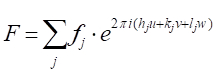
[9]
and the intensity factor contributed by the structure factor is I = F2.
Based on the positions (u,v,w) of atoms on particular planes (h,k,l), there is the possibility of interference between scattered waves that is constructive, destructive, or in-between, and this interference directly affects the amplitude of the XRD peaks representing the (hkl) planes.
Now, a plot of intensity, I, versus 2θ is what is measured in an XRD experiment. The determination of the of crystal type and the associated unit cell parameters (a, b, c, α, β, and γ) can be arrived at analytically by observing systematic presence/absence of peaks, using the equations 2-9, comparing values against databases, using deduction and a process of elimination. Nowadays, this is process is fairly automated by a variety of software linked to crystal structure databases.
PROCEDURE
The following procedure applies to a specific XRD instrument and its associated software, and there may be some variations when other instruments are used.
- We will examine a Ni powder sample on a Panalytical Alpha-1 XRD instrument.
- First, choose the mask to fix the beam size according to your sample diameter. The beam must not have a footprint larger than the sample at the smallest θ value (typically ~ 70-100). For a sample of width ε, the beam size should be < ε sinθ.
- Load the sample in the sample spinner stage and lock the sample into position. The sample spinner helps to spatially randomize the exposure of the sample to the X-ray source.
- Choose the angle range for your XRD scan. For example 15-90 degrees is a typical range.
- Choose a step size, i.e. the increment in 2θ, and integration (counting) time. Generally a 0.05 degree step size and 4 seconds integration is the default for a wide angle scan.
- Once all the peak positions are determined through this initial scan, subsequent scans can focus on a narrower scan range around specific peaks using a smaller step size in angle if higher resolution data from those peaks are desired.
RESULTS
In Figure 4 we see the XRD peaks for the Ni powder sample. Note that the peaks that are observed (e.g. {111}, {200}) are for those that have either all even or all odd combinations of h, k, and l. Ni is face-centered cubic (FCC), and in all FCC structures, the peaks corresponding to {hkl} planes where h, k, and l are mixtures of even and odd integers, are absent due to the destructive interference of the scattered X-rays. Peaks corresponding to planes, such as {210} and {211} are missing. This phenomenon is called the systematic presence and absence rules, and they provide an analytical tool for assessing the crystal structure of the sample.
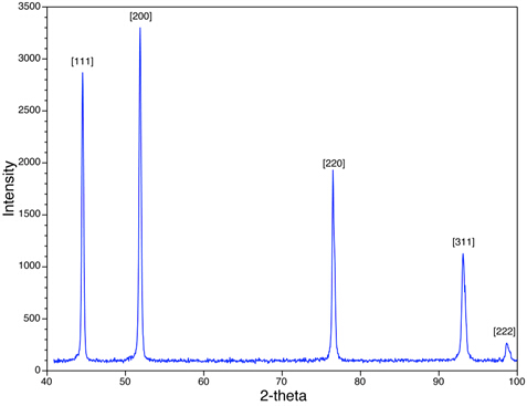
Figure 4: An XRD scan of Ni with a face-centered cubic structure is shown.
APPLICATIONS AND SUMMARY
This is a demonstration of a standard XRD experiment. The material examined in this experiment was in a powder form, but XRD works equally well with solid piece of material as long as the sample has a flat surface that can be set parallel to the plane of the sample stage.
XRD is a fairly ubiquitous method for determining the presence (or absence) of crystallographic order in materials. Beyond the standard application of determining the crystal structure, XRD is often used to obtain a variety of other structural information such as:
- Whether or not the structure of a material is amorphous (characterized by a broad hump in the diffraction intensity and a lack of discernable crystallographic peaks),
- Whether the sample is a composite material consisting of multiple crystallographic phases and, if so, determine the fraction of each phase,
- Determining whether a material is an amorphous/crystalline composite
- Determining the grain/particle size of the material,
- Determining the degree of texture (preferred orientation of grains) in material